 Contrary to what the image suggests, this article is about the born again shell, aka BASH. BASH is essential in any serious work on the GNU/Linux OS, which believe it or not is by far the most popular OS in the world, considering that the vast majority of servers run on it. Also, Linux-based OSes are popular among data scientists due to the versatility they offer, as well as their reliable performance. BASH is the way you interact with the computer directly when using a GNU/Linux system. In a way it is its own programming language, one that is on par with all the low-level languages out there, such as C. BASH is ideal for ETL processes, as well as any kind of automation. For example, the Cron jobs you may set up using Crontab are based on BASH. Of course, nothing beats a good graphical user interface (GUI) when it comes to ease-of-use, which is why most Linux-based OSes make use of a GUI too (e.g. KDE, Gnome, or Xfce). However, it's the command-line interface (CLI) that's the most powerful between the two. Also, the CLI is more or less the same in all Linux-based OSes and makes use of commands that are almost identical to those on the UNIX system. The programmatic framework of all this is naturally the BASH. BASH is not for the fainthearted, however. Unlike most programming languages used in data science (e.g. Python, Julia, Scala, etc.), BASH is not as easy to work with as it has an old-school kind of style. However, if you are proficient in any programming language, BASH doesn't seem so daunting. Also, scripts that are written in it as super fast and can do a lot of useful tasks promptly. Yet, even without getting your hands dirty with scripting on BASH, you can do a lot of stuff using aliases, which are defined in the .bash_aliases file. A cool thing about BASH is that you can call it through other programming environments too. In Julia, for example, you can either go directly to the shell using the semi-colon shortcut (;), or you can run a BASH command using the format run(`command`). Note that for this to work you need to use the appropriate character to define the command string (`). Interestingly, a lot of the commands in Julia are inspired by the BASH (e.g. pwd() is a direct reference to the pwd BASH command). So, if you are comfortable with Julia, you’ll find the BASH quite accessible too. Not easy, but accessible. Tools like BASH may not be easy to master (I’m still working on that myself, after all these years) but they can be useful even if you just know the basics. For example, it doesn’t take too much expertise to come up with a useful script that can speed up processes you normally use. For example, the RIP script I created recently can terminate up to three different processes that give you a hard time (yes, even in Linux-based OSes sometimes a process gets stuck!). Also, you can have another script to facilitate backups or even program updates and upgrades. The sky is the limit! All this may seem irrelevant to data science and A.I. work but the more comfortable you are with low-level programming like BASH, the easier it is to build high-performance pipelines, bringing your other programs to life. After all, you can’t get closer to the metal than with BASH, without using a screwdriver!
0 Comments
 Lately, I've been working with Julia a lot, partly because of my new book which was released a couple of weeks ago and partly because it's fun. If you are somewhat experienced with data handling, you'll probably familiar with the JLD and JLD2 packages that are built on top of the FileIO one. Of these, JLD2 is faster and generally better but it seems that it's no longer maintained, while the files it produces are quite bulky. This may not be an issue with a smaller dataset but when you are dealing with lots of data, it can be quite time-consuming to load or save data using this package. Enter the CDF framework, which is short for Compressed Data Format. This is still work in progress so don’t expect miracles here! However, I made sure it can handle the most common data types, such as scalars of any type (including complex string variables), the most common arrays (including BitArrays) for up to two dimensions, and of course dictionaries containing the above data structures. It does not support yet tensors or any kind of Boolean array (which for some bizarre reason is distinct from the BitArray data structure). CDF has two types of functions within it: those converting data into a large text string (and vice versa) and those dealing with IO operations, using binary files. The compression algorithm employed is the Deflate one from the CodecZlib package as it seems to have better performance than the other algorithms in the package. Remember that all of these algorithms take a text variable as an input, which is why everything is converted into a string before compressed and stored into a data file. The CDF framework doesn't have many of the options JLD2 has but for the files created with it, the performance edge is quite obvious. A typical dataset can be around 20 times smaller and many times faster to read or write, as the compression algorithm is fairly fast and there is fewer data to process with the computationally heavy IO commands. As a codebase, CDF is significantly simpler than other packages while the main functions are easy as pie. In fact, the whole framework is quite intuitive that there is not really any need for documentation for it. If you are interested in using this framework and/or extending it, feel free to contact me through this blog. Be sure to mention any affiliation(s) of yours too. Cheers!  Although it's fairly easy to compare two continuous variables and assess their similarity, it's not so straight-forward when you perform the same task on categorical variables. Of course, things are fairly simple when the variables at hand are binary (aka dummy variables), but even in this case, it's not as obvious as you may think. For example, if two variables are aligned (zeros to zeros and ones to ones), that’s fine. You can use Jaccard similarity to gauge how similar they are. But what happens when the two variables are reversely similar (the zeros of the first variable correspond to the ones of the second, and vice versa)? Then Jaccard similarity finds them dissimilar though there is no doubt that such a pair of variables may be relevant and the first one could be used to predict the second variable. Enter the Symmetric Jaccard Similarity (SJS), a metric that can alleviate this shortcoming of the original Jaccard similarity. Namely, it takes the maximum of the two Jaccard similarities, one with the features as they are originally and one with one of them reversed. SJS is easy to use and scalable, while its implementation in Julia is quite straight-forward. You just need to be comfortable with contingency tables, something that’s already an easy task in this language, though you can also code it from scratch without too much of a challenge. Anyway, SJS is fairly simple a metric, and something I've been using for years now. However, only recently did I explore its generalization to nominal variables, something that’s not as simple as it may first seem. Applying the SJS metric to a pair of nominal variables entails maximizing the potential similarity value between them, just like the original SJS does for binary variables. In other words, it shuffles the first variables until the similarity of it with the second variable is maximized, something that’s done in a deterministic and scalable manner. However, it becomes apparent through the algorithm that SJS may fail to reveal the edge that a non-symmetric approach may yield, namely in the case where certain values of the first variable are more similar toward a particular value of the second variable. In a practical sense it means that certain values of the nominal feature at hand are good at predicting a specific class, but not all of the classes. That's why an exhaustive search of all the binary combinations is generally better, since a given nominal feature may have more to offer in a classification model if it's broken down into several binary ones. That's something we do anyway, but this investigation through the SJS metric illustrates why this strategy is also a good one. Of course, SJS for nominal features may be useful for assessing if one of them is redundant. Just like we apply some correlation metric for a group of continuous features, we can apply SJS for a group of nominal features, eliminating those that are unnecessary, before we start breaking them down into binary ones, something that can make the dataset explode in size in some cases. All this is something I’ve been working on the other day, as part of another project. In my latest book “Julia for Machine Learning” (Technics Publications) I talk about such metrics (not SJS in particular) and how you can develop them from scratch in this programming language. Feel free to check it out. Cheers!  The concept of antifragility is well-established by Dr. Taleb and has even been adopted by the mainstream to some extent (e.g. in Investopedia). This is a vast concept and it’s unlikely that I can do it justice, especially in a blog post. That’s why I suggest you familiarize yourself with it first before reading the rest of this article. Antifragility is not only desirable but also essential to some extent, particularly when it comes to data science / AI work. Even though most data models are antifragile by nature (particularly the more sophisticated ones that manage to get every drop of signal from the data they are given), there are fragilities all over the place when it comes to how these models are used. A clear example of this is the computer code around them. I’m not referring to the code that’s used to implement them, usually coming from some specialized packages. That code is fine and usually better than most code found in data science / AI projects. The code around the models, however, be it the one taking care of ETL work, feature engineering, and even data visualization, may not always be good enough. Antifragility applies to computer code in various ways. Here are the ones I’ve found so far:
All this may seem like a lot of work and it may not agree with your temporal restrictions, particularly if you have strict deadlines. However, you can always improve on your code after you’ve cleared a milestone. This way, you can avoid some Black Swans like an error being thrown while the program you’ve made is already in production. Cheers! 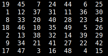 For over 2 decades there is a puzzle game I've played from time to time, usually to pass the time creatively or to challenge myself in algorithm development. This game, which I was taught by a friend, didn't have a name and I never managed to find it elsewhere so I call it Numgame (as it involves numbers and it's a game). Over the years, I managed to solve many of its levels though I never got an algorithm for it, until now. The game involves a square grid, originally a 10-by-10 one. The simplest grid that's solvable is the 5-by-5 one. The object of the game is to fill the grid with numbers, starting from 1 and going all the way to n^2, where n is the size of the grid, which can be any number larger than 4 (grids of this size or lower are not solvable). To fill the grid, you can "move" horizontally, vertically and diagonally, as long as the cell you go to is empty. When moving horizontally or vertically you need to skip 2 squares, while when you move diagonally you need to skip 1. Naturally, as you progress, getting to the remaining empty squares becomes increasingly hard. That's why you need to have a strategy if you are to finish the game successfully. Naturally, not all starting positions yield a successful result. Although more often than not you'd start from a corner, you may choose to start from any other square in the grid. That's useful, considering that some grids are just not solvable if you start from a corner (see image below; empty cells are marked as zeros) 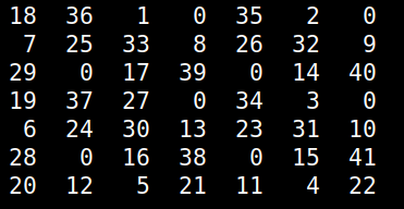 Before we look at the solution I've come across, try to solve a grid on your own and think about a potential algorithm to solve any grid. At the very least, you'll gain an appreciation of the solution afterward. Anyway, the key to solving the Numgame levels is to use a heuristic that will help you assess each move. In other words, you'll need to figure out a score that discerns between good and bad positions. The latter result from the various moves. So, for each cell in the grid, you can count how many legitimate ways are there for accessing it (i.e. ways complying with the aforementioned rules). You can store these numbers in a matrix. Then, you can filter out the cells that have been occupied already, since we won't be revisiting them anyway. This leaves us with a list of numbers corresponding to the number of ways to reach the remaining empty cells. Then we can take the harmonic mean of these numbers. I chose the harmonic mean because it is very sensitive to small numbers, something we want to avoid. So, the heuristic will take very low values if even a few cells start becoming inaccessible. Also, if even a single cell becomes completely inaccessible, the heuristic will take the value 0, which is also the worst possible score. Naturally, we aim to maximize this heuristic as we examine the various positions stemming from all the legitimate moves of each position. By repeating this process, we either end up with a full grid or one that doesn't progress because it's unsolvable. This simple problem may seem obvious now, but it is a good example of how a simple heuristic can solve a problem that's otherwise tough (at least for someone who hasn't tackled it enough to figure out a viable strategy). Naturally, we could brute-force the whole thing, but it's doubtful that this approach would be scalable. After all, in the era of A.I. we are better off seeking intelligent solutions to problems, rather than just through computing resources at them!  Lately, I've been busy with preparations for my conference trips, hence my online absence. Nevertheless, I found time to write something for you all who keep an open mind to non-hyped data science and A.I related content. So, this time I'd like to share a few thoughts on programming for data science, from a somewhat different perspective. First of all, it doesn't matter that much what language you use, if you have attained mastery of it. Even sub-Julia languages can be useful if you know how to use them well. However, in cases where you use a less powerful language, you need to know about lambda functions. I mastered this programming technique only recently because in Julia the performance improvement is negligible (unless your original code is inefficient to start with). However, as they make for more compact scripts, it seems like useful know-how to have. Besides, they have numerous uses in data science, particularly when it comes to:
Another thing that I’ve found incredibly useful, and which I mastered in the past few weeks, is the use of auxiliary functions for refactoring complex programs. A large program is bound to be difficult to comprehend and maintain, something that often falls into the workload of someone else you may not have a chance to help out. As comments in your script may also prove insufficient, it’s best to break things down to smaller and more versatile functions that are combined in your wrapper function. This modular approach, which is quite common in functional programming, makes for more useful code, which can be reused elsewhere, with minor modifications. Also, it’s the first step towards building a versatile programming library (package). Moreover, I’ve rediscovered the value of pen and paper in a programming setting. Particularly when dealing with problems that are difficult to envision fully, this approach is very useful. It may seem rudimentary and not something that a "good data scientist" would do, but if you think about it, most programmers also make use of a whiteboard or some other analog writing equipment when designing a solution. It may seem like an excessive task that may slow you down, but in the long run, it will save you time. I've tried that for testing a new graph algorithm I've developed for figuring out if a given graph has cycles (cliques) in it or not. Since drawing graphs is fairly simple, it was a very useful auxiliary task that made it possible to come up with a working solution to the problem in a matter of minutes. Finally, I discovered again the usefulness of in-depth pair-coding, particularly for data engineering tasks. Even if one's code is free of errors, there are always things that could use improvement, something that can be introduced through pair-coding. Fortunately, with tools like Zoom, this is easier than ever before as you don't need to be in the same physical room to perform this programming technique. This is something I do with all my data science mentees, once they reach a certain level of programming fluency and according to the feedback I've received, it is what benefits them the most. Hopefully, all this can help you clarify the role of programming in data science a bit more. After all, you don't need to be a professional coder to make use of a programming language in fields like data science. Throughout this blog, I've talked about all sorts of problems and how solving them can aid one's data science acumen as well as the development of the data science mindset. Problem-Solving skills rank high when it comes to the soft skills aspect of our craft, something I also mentioned in my latest video on O'Reilly. However, I haven't talked much about how you can hone this ability.
Enter Brilliant, a portal for all sorts of STEM-related courses and puzzles that can help you develop problem-solving, among other things. If you have even a vague interest in Math and the positive Sciences, Brilliant can help you grow this into a passion and even a skill-set in these disciplines. The most intriguing thing about all this is that it does so in a fun and engaging way. Naturally, most of the stuff Brilliant offers comes with a price tag (if it didn't, I would be concerned!). However, the cost of using the resources this site offers is a quite reasonable one and overall good value for money. The best part is that by signing up there you can also help me cover some of the expenses of this blog, as long as you use this link here: www.brilliant.org/fds (FDS stands for Foxy Data Science, by the way). Also, if you are among the first 200 people to sign up you'll get a 20% discount, so time is definitely of the essence! Note that I normally don't promote anything of this blog unless I'm certain about its quality standard. Also, out of respect for your time I refrain from posting any ads on the site. So, whenever I post something like this affiliate link here I do so after careful consideration, opting to find the best way to raise some revenue for the site all while providing you with something useful and relevant to it. I hope that you view this initiative the same way. 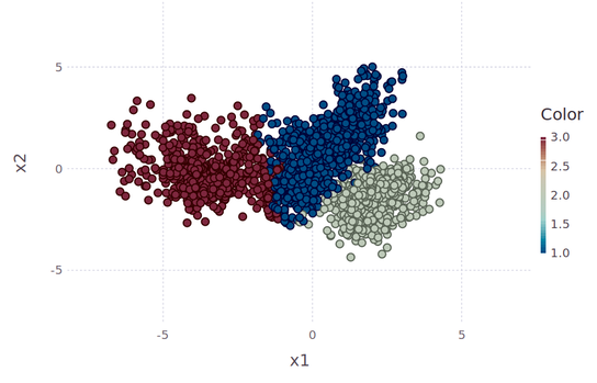 Short answer: Nope! Longer answer: clustering can be a simple deterministic problem, given that you figure out the optimal centroids to start with. But isn’t the latter the solution of a stochastic process though? Again, nope. You can meander around the feature space like a gambler, hoping to find some points that can yield a good solution, or you can tackle the whole problem scientifically. To do that, however, you have to forget everything you know about clustering and even basic statistics, since the latter are inherently limited and frankly, somewhat irrelevant to proper clustering.
Finding the optimal clusters is a two-fold problem: 1. you need to figure out which solutions make sense for the data (i.e. a good value for K), and 2. figure out these solutions in a methodical and robust manner. The former has been resolved as a problem and it’s fairly trivial. Vincent Granville talked about it in his blog, many years ago and since he is better at explaining things than I am, I’m not going to bother with that part at all. My solution to it is a bit different but it’s still heuristics-based. The 2nd part of the problem is also the more challenging one since it’s been something many people have been pursuing a while now, without much success (unless you count the super slow method of DBSCAN, with more parameters than letters in its name, as a viable solution). To find the optimal centroids, you need to take into account two things, the density of each centroid and the distances of each centroid to the other ones. Then you need to combine the two in a single metric, with you need to maximize. Each one of these problems seems fairly trivial, but something that many people don’t realize is that in practice, it’s very very hard, especially if you have multi-dimensional data (where conventional distance metrics fail) and lots of it (making the density calculations a major pain). Fortunately, I found a solution to both of these problems using 1. a new kind of distance metric, that yields a higher U value (this is the heuristic used to evaluate distance metrics in higher dimensional space), though with an inevitable compromise, and 2. a far more efficient way of calculating densities. The aforementioned compromise is that this metric cannot guarantee that the triangular inequality holds, but then again, this is not something you need for clustering anyway. As long as the clustering algo converges, you are fine. Preliminary results of this new clustering method show that it’s fairly quick (even though it searches through various values of K to find the optimum one) and computationally light. What’s more, it is designed to be fairly scalable, something that I’ll be experimenting with in the weeks to come. The reason for the scalability is that it doesn’t calculate the density of each data point, but of certain regions of the dataset only. Finding these regions is the hardest part, but you only need to do that once, before you start playing around with K values. Anyway, I’d love to go into detail about the method but the math I use is different to anything you’ve seen and beyond what is considered canon. Then again, some problems need new math to be solved and perhaps clustering is one of them. Whatever the case, this is just one of the numerous applications of this new framework of data analysis, which I call AAF (alternative analytics framework), a project I’ve been working on for more than 10 years now. More on that in the coming months.  Puzzles, especially programming related ones, can be very useful to hone one’s problem-solving skills. This has been known for a while among coders, who often have to come up with their own solutions to problems that lend themselves to analytical solutions. Since data science often involves similar situations, it is useful to have this kind of experiences, albeit in moderation. Programming puzzles often involve math problems, many of which require a lot of specialized knowledge to solve. This sort of problems, may not be that useful since it’s unlikely that you’ll ever need that knowledge in data science or any other applied field. Number theory, for example, although very interesting, has little to do with hands-on problems like the ones we are asked to solve in a data science setting. The kind of problems that benefit a data scientist the most are the ones where you need to come up with a clever algorithm as well as do some resource management. It’s easy to think of the computer as a system of infinite resources but that’s not the case. Even in the case of the cloud, where resource limitations are more lenient, you still have to pay for them, so it’s unwise to use them nilly-willy unless you have no other choice. Fortunately, there are lots of places on the web where you can find some good programming challenges for you. I find that the ones that are not language-specific are the best ones since they focus on the algorithms, rather than the technique. Solving programming puzzles won’t make you a data scientist for sure, but if you are new to coding or if you can use coding to express your problem-solving creativity, that’s definitely something worth exploring. Always remember though that being able to handle a dataset and build a robust model is always more useful, so budget your time accordingly.  Although there is a plethora of heuristics for assessing the similarity of two arrays, few of them can handle different sizes in these arrays and even fewer can address various aspects of these pieces of data. PCM is one such heuristic, which I’ve come up with, in order to answer the question: when are two arrays (vectors or matrices) similar enough? The idea was to use this metric as a proxy for figuring out when a sample is representative enough in terms of the distributions of its variables and able to reflect the same relationships among them. PCM manages to accomplish the first part. PCM stands for Possibility Congruency Metric and it makes use primarily of the distribution of the data involved as a way to figure out if there is congruency or not. Optionally, it uses the difference between the mean values and the variance too. The output is a number between 0 and 1 (inclusive), denoting how similar the two arrays are. The higher the value, the more similar they are. Random sampling provides PCM values around 0.9, but more careful sampling can reach values up closer to 1.0, for the data tested. Naturally, there is a limit to how high this value can get in respect with the sample size, because of the inevitable loss of information through the process. PCM works in a fairly simple and therefore scalable manner. Note that the primary method focuses on vectors. The distribution information (frequencies) is acquired by binning the variables and examining how many data points fall into each bin. The number of bins is determined by taking the harmonic mean of the optimum numbers of bins for the two arrays, after rounding it to the closest integer. Then the absolute difference between the two frequency vectors is taken and normalized. In the case of the mean and variance option being active, the mean and variance of each array are calculated and their absolute differences are taken. Then each one of them is normalized by dividing with the maximum difference possible, for these particular arrays. The largest array is always taken as a reference point. When calculating the PCM of matrices (which need to have the same number of dimensions), the PCM for each one of their columns is calculated first. Then, an average of these values is taken and used as the PCM of the whole matrix. The PCM method also yields the PCMs of the individual variables as part of its output. PCM is great for figuring out the similarity of two arrays through an in-depth view of the data involved. Instead of looking at just the mean and variance metrics, which can be deceiving, it makes use of the distribution data too. The fact that it doesn’t assume any particular distribution is a plus since it allows for biased samples to be considered. Overall, it’s a useful heuristic to know, especially if you prefer an alternative approach to analytics than what Stats has to offer. |
Zacharias Voulgaris, PhDPassionate data scientist with a foxy approach to technology, particularly related to A.I. Archives
December 2022
Categories
All
|
 RSS Feed