OK, this title may sound a bit heavy, especially for this time of year. Let me break it down for you. There are various correlation metrics out there, which can handle two variables (let's call them x and y) and measure their relationship. More often than not, these metrics focus on the linear aspects of this relationship and are often confused by the non-linear ones. For example, a correlation metric like Pearson’s Correlation can tell you that a variable y defined as 2x + 5 is strongly correlated to x (a shocker, isn't it!) but if a variable z is defined as exp(x^2 + 1) were to be used instead, well Pearson's Correlation might struggle with that. A mathematician or even a Stats professional would assure you that there is a non-linear relationship between the two variables (x and z), but they'd have to rely on a plot of the two variables or some transformation of one of them (e.g., applying log() to z) if they were to measure this relationship. Things get even more complicated if the relationship is not as simple, e.g. that of x and a variable w defined as cos(x). Most likely, Pearson's correlation won't find anything there (a relationship close to 0), even though the Math or Stats professional mentioned previously would be sure there is a relationship there. So, what gives?

Well, what gives is a big question that if I were to answer it here, it would shake your belief in Stats like a super quake, similar to that which brought San Francisco down over a century ago. Interestingly, most Stats concepts are from around that same time, perhaps a bit older than that. So, you've got to give those guys a break since they didn't know any better, plus they didn't have the tools we have at our disposal. Given the circumstances, they did a pretty good job at defining the metrics they did and weaving the fabric of a theory around their methods. Come to think about it, if modern mathematicians were like them, we'd be reasoning in high-dimensional terms now, instead of relying on these old-fashioned formulas and techniques.

I propose a method based on the BROOM framework that looks into the non-linear and non-monotonous artifacts of a pair of variables to establish their relationship. This metric, which I call rbc (range-based correlation, as it's part of the ranges part of the framework), explores the two variables in an entirely data-driven manner, making no assumptions whatsoever about their distributions and their other aspects. As long as they are normalized, they are good to go. And this metric, contrary to all other correlation metrics I've tried, yields a correlation of 0.99 for the x-w pair and a similar figure for the x-z one. When you compare x with some random variable q (q belongs to the [0, 1] interval), it yields a weak correlation (usually between 0.1 and 0.2). As a result, we can deduce that it's a worthwhile metric for measuring the relationship between two variables, taking into account all non-linear artifacts while being unaffected by any lack of a monotonous pattern the two variables may exhibit. If you are interested in learning more, feel free to contact me. Cheers!

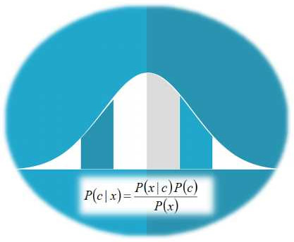
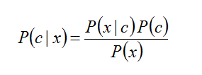
Everyone can analyze data these days, given the right programming tool and some library of functions, to express practically the relevant know-how of that person. I've seen people who give away books for free (as it would be impossible for them to get others to buy them) analyze data. As data science becomes more widespread, data analysis becomes a given for a larger portion of the population. But what about data synthesis, however? What's up with that? Let's delve into this.

First of all, let's get some definitions down. Data synthesis is the creation of synthetic data that follows a given pattern. The latter can be given directly to the data generation program, or it can be derived (extrapolated) via data analytics. Synthetic data is ideally indistinguishable from conventional data, and you can use it to train a data model, for example. However, there is something that makes it extremely valuable.

The value of synthetic data lies in the fact that it's not tied to particular individuals, so using this data doesn't pose any PII-related issues. Because of this, it cannot be owned by any specific person, even if it can be leveraged in the data science pipeline, yielding value. Naturally, since there are no shortcuts to value-making, the value (information) of that synthetic data must come from somewhere. So, since it's not practical for someone to have a high-level mathematical representation of this value and give it to a program as a pattern, it's more likely that this value stems from the source data.

So, to have valuable synthetic data (that's also free of PII), we need to have some source data of value, for starters. That's why the only practical way to generate synthetic data that's worth its space on a hard disk is via analytics. Of course, there are ways to generate such data through analytics, as in the case of some specialized deep learning networks (Autoencoders). The catch is that these A.I. systems require lots of data to do their job. After all, analyzing multiple variables isn't easy, even for an A.I. What if there was a way to perform the same task without employing these more advanced data-hungry systems?

Enter the BROOM framework again! We've already described some of its functionality, but what if this was just a prelude for its more sophisticated aspects? Well, fortunately, data synthesis isn't all that different from sampling, if you know what you are doing? And if you can sample a dataset properly, it's not that much more challenging to create new data points aligned with its essence. Naturally, the synthetic data is generated in a stochastic manner since it makes more sense to leverage noise in this process. Otherwise, all the generated data would be the same every time. Oh, and did I mention that this data synthesis process is scalable to as many dimensions as you like? Because if you understand data in-depth, the cardinality of vectors in a dataset is just another number...

I've been trying to answer this question for years. Well, not many years, but still, at least since the second half of the previous decade. Why? Well, I've always liked to explore the boundaries between the continuous and the discrete and since I finally internalized the teaching that everything in this universe is discrete (see: Quantum Physics), I decided to explore that angle and see if there was indeed a way to turn a continuous variable into a discrete one, with minimal information loss.

Over the past few months, I've developed three distinct approaches, depending on how distinct the values of the target variable are (see what I did there?). Let's start with something simple: no target variable at all. So, how can we discretize a continuous variable x? Well, you have to binarize it until there is no more binarization possible! But how do you optimally binarize a variable? That's something that involves densities after you handle all outliers and inliers in x, of course. How do you do that? Well, that's a topic that can fill a whole book chapter, so I'll have to draw the line here, I'm afraid.

What about when there is a target variable? Let's start with a binary one as it's simpler this way. We can employ a robust similarity metric that can assess the similarity of two binary variables, regardless of their alignment or any similarities due to chance. Fortunately, I've developed one such metric, which I call holistic symmetric similarity (HSS), which also works with all sorts of discrete variables. So, by using this metric, we can optimize the split to maximize the HSS score between the binarized x and the target variable y. The same approach works if y is discrete but not binary since I've generalized HSS to handle nominal variables too. 

Ok, but what about when y is continuous, though? Well, that takes a bit more creativity since it's not as simple a task as it may seem. Fortunately, it's doable and relatively light, computationally speaking. We can find the threshold that maximizes a custom correlation metric that becomes larger once any non-linearities are tackled. This process doesn't have to be rocket science since I'm sure you can come up with a metric like that if you've been mentored by someone worth his salt in data science. Of course, you could use a translinearity correlation metric, yet, I wouldn't recommend that since it would inevitably pick up signals you wouldn't want it to, plus it's bound to be more computationally heavy. 

So, there you have it. You can binarize and therefore discretize any feature x you like, with or without a target variable. The latter can be binary, discrete, or even continuous, depending on the problem at hand. Such a process can help you preserve computational resources and perhaps even enable you to make better and more transparent models (after all, binary variables tend to be easier on the mind, not just on the computer). All this I've done in the OD.jl script, which I cannot share here, unfortunately, as it has dependencies on proprietary code (the BROOM framework), which I'd rather not give away. Still, if you wish to explore this topic further, we can do that in a one-on-one mentoring session or two, given that you have the required commitment to the craft and a genuine interest to learn more about it. Cheers!

A-B testing plays a crucial role in traditional science as well as data science. It isn't easy to imagine a scientific experiment worth its time without A-B testing. It's such a useful technique that it features heavily in data analytics too. In this article, we'll explore this essential method of data analysis, focusing on its role in scientific work and data science.

In a nutshell, A-B testing uses data analysis to determine if two different samples are significantly different from each other, concerning a given variable. The latter is usually a continuous variable, used to examine how different the two samples are (it can be nominal too, however). The two samples often derive from a partitioning of a dataset based on another variable, which is binary. A-B testing is closely linked to Statistics, although any heuristic could be used to evaluate the difference between the two samples. Still, since Statistics yields a measurable and easy-to-interpret result in the form of a probability (p-value), it's often the case that particular statistical tests are used for A-B testing.

A-B testing is used heavily in scientific work. The reason is simple: since there are several hypotheses the analyst considers, it's often the case that the best way to test many of these hypotheses is through A-B testing. After all, this methodology is closely linked to the formation of a hypothesis and its testing, based on the data at hand. Naturally, the usefulness of A-B testing is also apparent in data science and data analytics during the data exploration stage.

The statistical tests used for A-B testing are t-tests, chi-square tests, and to a lower extent, z-tests. The t-test handles cases where a continuous variable is involved (e.g., Sales), while the chi-square one is geared towards nominal variables. Z-tests are very much like t-tests, but they are less powerful and make stronger assumptions about the data. All statistical tests yield a p-value as a result, which is compared to a predefined threshold (alpha), taking values like 0.05, 0.01, or 0.001. The lower the p-value, the more significant the result. Having a p-value lower than the alpha value means that you can safely disprove the Null Hypothesis (which states that any differences between the two samples are due to chance).

Note that A-B testing is a deep topic, and it's hard to do it justice in a blog article. Also, it requires a lot of practice to understand it thoroughly. So, if it sounds a bit abstract, that's normal, especially if you are new to Statistics. Cheers!

Data analytics is the field that deals with the analysis of data, usually for business-related objectives, though its scope covers any organization. A data analyst handles data with various tools, such as a spreadsheet program (usually MS Excel), a data visualization program (e.g. Tableau), a database program (e.g. PostgreSQL), and a programming language (usually Python), and then presents her findings using a presentation program (e.g. MS PowerPoint). This aids business decisions and provides useful insights into the state of an organization. It's akin to the Business Intelligence role, though a bit more hands-on and programming-related.

What about Statistics though? Well, it is a potent data analytics tool but whether it's something a data analyst actually needs is quite debatable. Apart from some descriptive stats that you are bound to use in one way or another, the bulk of Statistics is way too specialized and irrelevant to a data analyst. It doesn't hurt knowing it but it would highly biased to promote this sort of knowledge (in most cases it doesn't even classify as know-how) when there are much more efficient and effective tools out there. For example, being about to handle the data coming from various sources and organize it, be it through an ETL tool or some data platform, is far more of a value-add than trying to do something that's often beyond the scope of your role as an analyst (e.g. an in-depth analysis of the data at hand, through advanced data engineering or predictive modeling).

Having said that, Statistics is useful in data science, particularly if you are not well-versed in more advanced methodologies, such as machine learning. That’s why most data science courses start with this part of the toolbox along with the corresponding programming libraries. Also, most time-series analysis models are Stats-based and data scientists are often required to work with them, at least as a baseline before proceeding to build more complex models. Moreover, if you want to test a hypothesis (something quite common in data science work), you need to make use of statistical tests.

In data analytics, however, where the objective is somewhat different, Stats seems to be a somewhat unnecessary tool. Perhaps that's why most data analysts focus on other more practical and guaranteed ways to add value, such as dashboards, intuitive spreadsheets, and useful scripts, rather than building statistical models that few people care about. Besides, if someone needs something more in-depth and scientifically sound, they can always hire a couple of data scientists to work alongside with the analysts.

Regardless of your role, you can learn more about data science and the mindset behind it in my book Data Science Mindset, Methodologies, and Misconceptions. Although it was published about 4 years ago, it remains relevant and can shed a lot of light on Statistics' role in this field, as well as other methodologies and tools used by data scientists. Check it out when you have some time. Cheers!

Nowadays, there is a lot of confusion between the fields of Statistics and Machine Learning, which often hinders the development of the data science mindset. This is especially the case when it comes to innovation since this confusion can often lead someone to severe misconceptions about what's possible and the value of the data-driven paradigm. This article will look into this topic and explore how you can add value through a clearer understanding of it.

First of all, let's look at what statistics is. As you may recall, statistics is the sub-field that deals with data from a probabilistic standpoint. It involves building and using the mathematical models that describe how the data is distributed (distributions) and figuring out the likelihood of data points being part of these distributions through these functions. Many heuristics are used, though they are called statistic metrics or just statistics, and the whole field is generally very formalist. When data behaves as expected and when there is an abundance of it, statistics works fine, while it also yields predictive models that are transparent and easy to interpret or explain.

Now, what about machine learning? Well, this is a field of data analytics that involves an alternative approach to handling data, one that's more data-driven. In other words, machine learning involves analyzing the data without any ad-hoc notions about it, in the form of distributions or any other mathematical frameworks. That's not to say that machine learning doesn't involve math, far from it! However, the math in this field is used to analyze the data through heuristic-based and rule-based models, rather than probabilistic ones. Also, machine learning ties in very well with artificial intelligence (A.I.), so much so that they are often conflated. A.I. has a vital role in machine learning today, so the AI-based models often dominate in this field.

As you may have figured out by now, the critical difference between statistics and machine learning lies in the fact that statistics makes assumptions about the data (through the distribution functions, for example) while machine learning doesn't. This difference is an important one that makes all the difference (no pun intended) in the models' performance. After all, when data is complex and noisy, machine learning models tend to have better performance and generalize better. Perhaps that's why they are the most popular option in data science projects these days.

You can learn more about the topic by checking out my latest book, which covers machine learning from a practical and grounded perspective. Although the book focuses on how you can leverage Julia for machine learning work, it also covers some theoretical concepts (including this topic, in more depth). This way, it can help you cultivate the right mindset for data science and broaden your perspective on the data science field. So, check it out when you have a moment!

Statistics is a very interesting field that has some relevance to data science work. Perhaps not as much as some people claim, but it's definitely a useful toolset, particularly in the data exploration part of the pipeline. But how can Stats improve, particularly when it comes to new technologies like A.I.?

Statistics can benefits from such technologies in various ways. The most important is the mindset of the AI-based approach, which is empirical and pragmatic. Instead of imagining complex theories for explaining the data, AI looks at it as it is and works with it accordingly (the data-driven approach).

Conventional Statistics on the other hand tries to fit the data into this or the other mathematical model for describing it and then it processes the data with some arbitrary metrics that are mediocre at best. However, the math is elegant, so we go with it anyway. So many textbooks can’t be wrong, right? Well, in data science there is no right or wrong, just models that work well and others that don’t work as well. Since there is usually money on the line, we prefer to go with the former models, which coincidentally tend to be machine learning related, particularly AI-based. So, there is surely room for improvement for Statistics if it were to adopt the same mindset.

What's more, Statistics can benefit from A.I. through additional heuristics (or statistics, as they are often referred to in that context). The existing heuristics may work well, but they are very narrowly defined, making them overly specialized. AI-based heuristics are broader and tend to be more applicable in a variety of data sets. If Statistics were to adopt a similar approach to heuristics, it would for sure benefit greatly and become more widely applicable.

Finally, Statistics can benefit from A.I. by embracing a different approach to describing the data. This is a more fundamental change and probably most fans of the field will disregard it as impractical. However, it is feasible and even efficient, with a bit of clever programming (based on heuristics and a geometrical approach). The latter is something Statistics seems to be divorced from, which is another area of improvement.

It's worth noting that although developments in Statistics are bound to be beneficial to anyone applying it in data analytics projects, the practitioner also needs to evolve. There is no point in advancing this field if its practitioners remain in their old ways, limited and rigid. Perhaps that's one of the reasons machine learning and A.I. have advanced so much; their practitioners are more open to changes and willing to adapt. No wonder these fields now dominate the data science world. Something to think about...

PS - This article was supposed to be published yesterday. However, there was an issue with the scheduler, hence the delay. Normally, I'll have new material every Monday and sometimes on Thursdays too. Cheers!

Even if you are not a Bayesian Stats fan, it’s not hard to appreciate this data analytics framework. In fact, it would irresponsible if you were to disregard it without delving into it, at least to some extent.  Nevertheless, the fact is that Frequentist Stats (see image above), as well as Machine Learning, are more popular in data science. Let's explore the reasons why this is.

Bayesian Stats relies primarily on the various versions of the Bayes Theorem. In a nutshell, this theorem states that if we have some idea of the a priori probabilities of an event A happening (as well as A not happening), as well as the likelihoods of event B happening given event A happening (as well as A not happening), we can estimate the probability of A given B. This is useful in a variety of cases, particularly when we don't have a great deal of data at our disposal. However, there is something often hard to gauge and it's the Achilles heel of Bayesian Stats. Namely, the a priori probabilities of A (aka the priors) are not always known while when they are, they are usually rough estimates. Of course, this isn't a showstopper for a Bayesian Stats analysis, but it is a weak point that many people are not comfortable with since it introduces an element of subjectivity to the whole analysis.

In Frequentist Stats, there are no priors and the whole framework has an objective approach to things. This may seem a bit far-fetched at times since lots of assumptions are often made but at least most people are comfortable with these assumptions. In Machine Learning, the number of assumptions is significantly smaller as it's a data-driven approach to analytics, making things easier in many ways.

Another matter that makes Bayesian Stats not preferable for many people is the lack of proper education around this subject. Although it predates Frequentist Stats, Bayesian Stats never got enough traction in people's minds. The fact that Frequentist Stats was advocated by a very charismatic individual who was also a great data analyst (Ronald A. Fisher) may have contributed to that. Also, the people who embraced the different types of Statistics at the time augmented the frameworks with certain worldviews, making them more like ideological stances than anything else. As a result, since most people who worked in data analytics at the time were more partial towards Fisher's worldview, it made more sense for them to advocate Frequentist Stats. The fact that Thomas Bayes was a man of the cloth may have dissuaded some people from supporting his Statistics framework.

Finally, Bayesian Stats involves a lot of advanced math when it is applied to continuous variables. As the latter scenario is quite common in most data analytics projects, Bayesian Stats ends up being a fairly esoteric discipline. The latter entails things like Monte Carlo simulations (which although fairly straightforward, they are not as simple as distribution plots and probability tables) and Markov Chains. Also, there are lots of lesser-known distributions used in Bayesian Stats (e.g. Poisson, Beta, and Gamma, just to name a few) that are not as simple or elegant as the Normal (Gaussian) distribution or the Student (t) distribution that are bread and butter for Frequentist Stats. That's not to say that the latter is a walk in the park, but it's more accessible to a beginner in data analytics. As for Machine Learning, contrary to what many people think, it too is fairly accessible, especially if you use a reliable source such as a course, a book, or even an educational video, etc. with a price tag accompanying it.

Summing up, Bayesian Statistics is a great tool that’s worth exploring. If, however, you find that most data analytics professionals don’t share your enthusiasm towards it, don’t be dismayed. This is something natural as the alternative frameworks maintain an advantage over Bayesian Stats.

Lately, there has been a lot of talk about the Corona Virus disease (Covid-19) and Italy is allegedly a hotspot. As my partner lives in Italy and is constantly bombarded by warnings about potential infections and other alarming news like that, I figured it would be appropriate to do some back-of-the-envelop calculations about this situation and put things in perspective a bit. After all, Bologna (the city where she lives) is not officially a "red zone" like Milan and a few other cities in the country.

For this analysis, I used Bayes' Theorem (see formula below) along with some figures I managed to dig up, regarding the virus in the greater Bologna area. The numbers may not be 100% accurate but they are the best I could find, while the assumption made was more than generous.

Namely, I used the latest numbers regarding the spread of the disease as the priors, while regarding the likelihoods (conditional probabilities regarding the test made) I had to use two figures, one from the Journal of Radiology to figure out the false positives rate (5 out of 167 or about 3%, in a particular study) and one for the true positive rate (aka precision), the aforementioned assumption, namely 99%. In reality, this number is bound to be lower but for the sake of argument, let's say that it's correct 99% of the time. Note that certain tests regarding the Covid-19 using CT scans can be as low as 80%, while the test kits available in some countries have even lower precision. For the priors, I used the data reported in the newspaper, namely around 40 for the greater Bologna area. The latter has a population of about 400 000 people (including the suburbs). So, given all that, what are the chances you actually have the virus if you do a test for it the result comes back positive?

Well, by doing the math on Bayes’ theorem, it can take the form:
P(infection | positive) = P(positive | infection) * P(infection) / [P(positive | infection) * P(infection) + P(positive | healthy) * P(healthy)]

As being infected and being healthy are mutually exclusive, we can say that P(healthy) = 1 – P(infection). Doing some more math on this we end up with this slightly more elegant formula:
P(infection | positive) = 1 / [1 + λ (1 / P(infection) – 1)] where λ = P(positive | healthy) / P(positive | infection).
Plugging in all the numbers we end up with: P(infection | positive) = 1 / (1 + 303) = 0.3% (!)

In other words, even if you do a proper test for Covid-19, and the test is positive (i.e. the doctor tells you “you’re infected”) the chances of this being true are about 1 in 300. This is roughly equivalent to rolling a triple 1 using 3 dice (i.e. you roll three dice and the outcome is 1-1-1). Of course, if you don’t test positive, the chances of you having the virus are much lower.

Note that the above analysis is for the city of Bologna and that for other cities you'll need to update the formula with the numbers that apply there. However, even if the scope of this analysis is limited to the greater Bologna area, it goes on to show that this whole situation that plagues Italy is more fear-mongering than anything else. Nevertheless, it is advisable to be mindful of your health as during times of changing weather (and climate), your immune system may need some help to ensure it keeps your body healthy, so anything you do to help it is a plus. Things like exercise, a good diet, exposure to the sun, keeping stress at bay, and maintaining good body hygiene are essential regardless of what pathogens may or may not threaten your well-being. Stay healthy!

(image by Arek Socha, available at pixabay)

Lately, I've been working on the final parts of my latest book, which is contracted for the end of Spring this year. As this is probably going to be my last technical book for the foreseeable future, I'd like to put my best into it, given the available resources of time and energy. This is one of the reasons I haven't been very active on this blog as of late. In this book (whose details I’m going to reveal when it’s in the printing press) I examine various aspects of data science in a quite hands-on way. One of these aspects, which I often talk about with my mentees, is that of scale.

Scaling is very important in data science projects, particularly those involving distance-based metrics. Although the latter may be a bit niche from a modern standpoint where A.I. based systems are often the go-to option, there is still a lot of value in distances as they are usually the prima materia of almost all similarity metrics. Similarity-based systems, aka transductive systems, are quite popular even in this era of A.I. based models. This is particularly the case in clustering problems, whereby both the clustering algorithms and the evaluation metrics (e.g. Silhouette score/width) are based on distances for evaluating cluster affinity. Also, certain dimensionality reduction methods like Principle Components Analysis (PCA) often require a certain kind of scaling to function optimally.

Scaling is not as simple as it may first seem. After all, it greatly depends on the application as well as the data itself (something not everyone is aware of since the way scaling/normalization is treated in data science educational material is somewhat superficial). For example, you can have a fixed range scaling process or a fixed center one. You can even have a fixed range and fixed center one at the same time if you wish, though it's not something you'd normally see anywhere. Fixed scaling is usually in the [0, 1] interval and it involves scaling the data so that its range is constant. The center point of that data (usually measured with the arithmetic mean/average), however, could be distorted. How much so depends on the structure of the data. As for the fixed center scaling, this ensures that the center of the scaled variable is a given value, usually 0. In many cases, the spread of the scaled data is fixed too, usually by setting the standard deviation to 1.

Programmatic methods for performing scaling vary, perhaps more than the Stats educators will have you think. For example, in the fixed range scaling, you could use the min-max normalization (aka 0-1 normalization, a term that shows both limited understanding of the topic and vagueness), or you could use a non-linear function that is also bound by these values. The advantage of the latter is that you can mitigate the effect of any outliers, without having to eradicate them, all through the use of good old-fashioned Math! Naturally, most Stats educators shy away at the mention of the word non-linear since they like to keep things simple (perhaps too simple) so don’t expect to learn about this kind of fixed-range scaling in a Stats book.

All in all, scaling is something worth keeping in mind when dealing with data, particularly when using a distance-based method or a dimensionality reduction process like PCA. Naturally, there is more to the topic than meets the eye, plus as a process, it's not as basic as it may seem through the lens of package documentation or a Stats book. Whatever the case, it's something worth utilizing, always in tandem with other data engineering tools to ensure a better quality data science project.