Is Urbanization a Phenomenon Predictable by the Per Capita Income in a Nation, Subject to the Hemisphere It Belongs to? A Case Study Using Python.

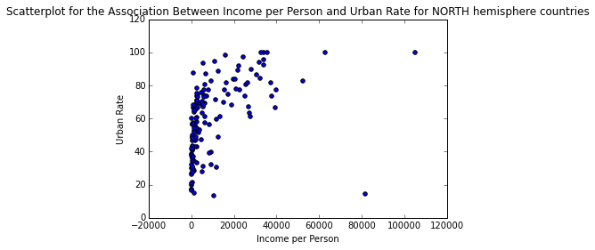
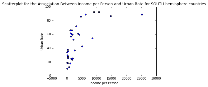
In the previous case studies we examined various socio-economical attributes for the registered countries in Gapminder. Yet, our analyses were somewhat superficial, since we didn’t look into moderating variables that may influence the end result, since the relationships among the variables are more like a web than a simple set of independent connections. This case study is an attempt to unravel this web by examining how the “hemisphere” variable moderates the relationship between per capita income (incomeperperson variable) and urban rate. To do this we need to employ an analysis suitable for numeric vs. numeric variables, such as Pearson Correlation, but...

Once we import the data from the enriched data file (see 2nd case study for details on how we did this) to a data frame called “data”, we convert the variables of interest to numeric and isolate them, along with the “hemisphere” categorical variable in a data frame called “subframe”. Then we take care of all the missing values (blank in the case of incomeperperson and urbanrate and “NA” in the case of hemisphere) and store the processed data set in the data frame “clean_data”. Then we partition the data frame into two mutually exclusive ones, depending on the value of the “hemisphere” variable, namely one data frame for the North hemisphere and one for the South. Next we calculate the associations between Income per Person and Urban Rate for each hemisphere, using the Pearson’s Correlation metric. The resulting index and corresponding p-value for each hemisphere are as follows:

North: (0.48338796757916214, 6.4066230298988046e-10)
South: (0.67386547341458669, 6.6362307251623208e-06)

So, for the North hemisphere it appears that these two variables are associated positively but in a weak way. Nevertheless, this is a very significant relationship, since the p-value is extremely small (<<0.001). For the South hemisphere the relationship is also positive but much larger (borderline strong) while being very significant too (though not as significant, probably due to the fact that there are much fewer countries in the South hemisphere). These relationships are reflected in the plots below:

One important caveat of this analysis is that the Pearson Correlation fails to reflect the actual relationship between Income per Person and Urban Rate variables, which based on the plots is logarithmic in nature. So, even though the metric shows that it’s weak, it merely states that there isn’t a strong linear connection between the variables. Nevertheless, this case study clearly illustrates the presence of a moderating variables in this relationship, namely the hemisphere one.

As always, you can review the data and the code used in this analysis using the attachments below.

gapminder_with_hemispheres.csv
File Size:	26 kb
File Type:	csv

Download File

---

assignment_4_py.txt
File Size:	1 kb
File Type:	txt

Download File

---